5 CBM_core
This documentation is work in progress. Potential discrepancies and omissions may exist for the time being. If you find any, please contact us here.
5.1 Overview
CBM_core is the central module of spadesCBM. This is where all the carbon transfers are calculated at every time step, where disturbances are applied, and stocks are tracked. It cannot run on its own and it needs parameters from CBM_defaults, CBM_dataPrep_SK, CBM_dataPrep, and CBM_vol2biomass (as per the provided example for managed forests of Saskatchewan) or the equivalent information from the user. In SpaDES-speak, this module has six events (Init, spinup, annual_preprocessing, annual_carbonDynamics, save, and plot). Only in two of these events do carbon transactions occur: spinup and annual_carbonDynamics. The other events are tools to enable these transactions. All events are scheduled only once except for the two annual events, who schedules themselves until the end of the simulation horizon. Only in this module are the Python functions from the libcbm package called. The functions used in this module are the libcbm cbm-exn functions exclusively, as these were designed to accept external biomass increments. These Python functions are used in the spinup and in the annual_carbonDynamics events only.
5.2 Background
In CBM_core, the approach described in our Overview section is applied. Parameters are easily accessible via normal R-functions, and the SpaDES toolkit enables a modular, repeatable continuous workflow. This brings the transparency and flexibility needed for scientists to modify, evaluate and test new inputs, new data, and new algorithms while permitting non-researcher users to also use the system.
5.3 Inputs
| Name | Class | Description | Source |
|---|---|---|---|
| growth_increments | Data table | growth increment matrix | CBM_vol2biomass |
| standDT | Data table | Table of stand attributes. Stands can have 1 or more cohorts | CBM_dataPrep |
| cohortDT | Data table | Table of cohort attributes | CBM_dataPrep |
| masterRaster | SpatRaster | Raster of study area | User provided, for SK: Google Drive |
| gcMeta | Data table | Growth curve metadata | CBM_dataPrep |
| pooldef | Character | Vector of pools | CBM_defaults |
| spinupSQL | Data table | Parameters for CBM_core spinup event | CBM_defaults |
| disturbanceEvents | Data table | Table with disturbance events for each simulation year | CBM_dataPrep |
| disturbanceMeta | Data table | Table defining disturbance event types | CBM_dataPrep_SK |
5.4 Module functioning
5.4.1 Events
There are 6 main events in CBM_core. Each are run once, except for the annual_X events, which are repeated for each simulation year.
5.4.1.1 Init
In this short event, the Python virtual environment is set up. If a suitable version of python is not available, it will be installed using the reticulate package.
5.4.1.2 spinup
The main goal of this event is to initialize the landscape by performing the spinup function.
Cohort and stand data is prepared and passed to the cbmExnSpinup function alongside growth curve data (from CBM_vol2biomass) and spinup default data (from CBM_defaults). The cbmExnSpinup function sets up inputs, calls the cbm_exn_get_default_parameters python function that defines the model structure, and runs the carbon transfers necessary for the growth and burn cycle using cbm_exn_spinup.
The spinup output data and cohort groups are then prepared for use in the annual event.
5.4.1.3 annual_preprocessing
This event serves to run 2 smaller events: annual_prepDisturbances and annualprepCohortGroups. The first reads in and saves the disturbances for the current simulation year for processing in the annual_carbonDynamics event. The latter prepares cohort data for the upcoming carbon dynamics processing. It saves old and sets new group IDs for disturbed pixels, clears information about previous disturbances, prepares data for new cohort groups, removes inactive groups, and sets the appropriate growth increments for the current simulation year.
5.4.1.4 annual_carbonDynamics
This event is where all the carbon transfers are applied for each simulation year. Disturbances are matched to the correct records, and the transfers listed here are applied. Details on transfer rates are found in the following section, below. While undisturbed cohorts will continue to grow by one time step according to their associated growth curve, disturbed cohorts will only begin growing again after a delay period. This delay is dictated by the default_delay_regen parameter of the CBM_core module, and can be changed by the user. Only growth-related carbon transfers are affected by this delay. By default it is set to 0 years.
5.4.1.5 save
This event is where outputs are saved. In the case of our example in Saskatchewan, we save outputs to .qs files to our spadesCBMdb object for each simulation year. By default, 3 tables are saved, a key table, a pools table, and a flux table. Other tables with simulation parameters can be saved by changing the .saveAll parameter to TRUE in the module. If output paths are kept at default, hese output files will be found here: ~/GitHub/spadesCBM/outputs.
5.4.1.6 plot
This final event is where all plotting occurs. Plots will be saved as .png files in the project’s outputs folder. Similar to in accumulateResults, if paths are kept at default when running our example global script, these outputs will be found here:
~/GitHub/spadesCBM/outputs. You can also view examples of these plots here.
5.4.2 Stands and Cohort Groups
Cohort groups are unique combinations of age, growth curve (which equates to species as there is one growth curve per leading species in CBM), spatial unit and ecozone. In spadesCBM, forested pixels are simulated and represent a stand. Each stand (or pixel) can have one or many cohorts. All cohorts across stands that share an identical age, growth curve, spatial unit, and ecozone will share one unique cohortGroupID number.
The object allPixDT is a large table with a row corresponding to every pixel in the masterRaster. The cohortDT object is a long-form table where each simulated pixel (or stand) has its own row (no NAs), and cohortGroups lists only the cohort groups and their attributes. In our example there are 1 347 529 pixels simulated (i.e., 1 347 529 rows in cohortDT) which are grouped in 739 cohortGroups for processing (i.e. 739 rows in cohortGroups).
5.4.3 Carbon Transfers
Default parameters for simulations are available mainly from default .csv files with a few pieces of information such as mean_annual_temperature used in decay rates calculations, return_interval, min_rotations and max_rotations used in the spinup or initialization process available in an SQLite database. There are 18 internal carbon pools in spadesCBM (see Table 1 in Overview), and two pools that take carbon out of the system, one for the atmosphere and one for harvested wood exiting the system. Disturbances are the first carbon transfer to be applied to each record. Half the annual increment is then added (transfer from the atmosphere to the three above ground biomass pools - Merch, Foliage, and Other). Disturbance inputs are processed externally to CBM_core. In our example disturbances are processed in CBM_dataPrep_SK, leaving CBM_core free of spatial data manipulations. Disturbance matrices specify the proportion of carbon in each pool to be transferred to other pools or to be taken out of the system (via forest products (pool named Products) or back to the atmosphere). Figure 1 gives an example of transfers during a fire in Saskatchewan.
Figure 1: Proportional carbon transfers between pools during a fire in Saskatchewan
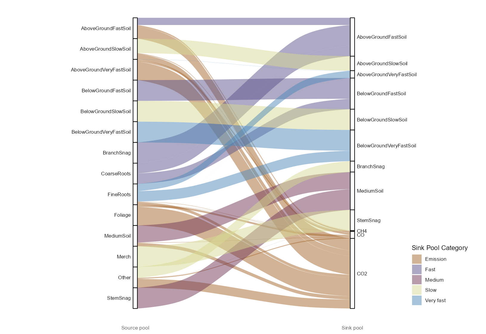
The amount of carbon transferred from the atmosphere to the above ground biomass pools is determined from the growth curves, which were translated from \(m^3/ha\) to carbon increments in CBM_vol2biomass and provided to CBM_core in carbon increments (in tonnes of carbon/ha). In our example the object simMngedSK$growth_increments has the increments used for the simulation. Dead Organic Matter (DOM) turnover happens next and transfers carbon from the pools representing snags (StemSnags and BranchSnags), to the MediumSoil, and AboveGroundFastSoil pools. Biomass turnover follows with transfers from the Merch, Foliage, Other, FineRoots and CoarseRoots, to the pools representing the snags (StemSnags and BranchSnags), AboveGroundVeryFastSoil, BelowGroundFastSoil, AboveGroundVeryFastSoil and BelowGroundVeryFastSoil pools. Carbon is never lost in the system, but increments are at times negative. To accommodate negative increment values, a carbon transfer labelled overmature_decline, moves carbon between the Merch, Other, Foliage, CoarseRoots and FineRoots to pools representing stem an branch snags, and the AboveGroundFastSoil, AboveGroundVeryFastSoil, BelowGroundFastSoil, and BelowGroundVeryFastSoil pools. The transfers are portioned in the same way as the annual turnover and the amount is equal to the loss of each individual biomass pool according to the negative increment. Following the overmature_decline transfers, the second half of the growth is added to the three above ground biomass pools - Merch, Foliage, and Other. Next, the transfers due to decay are performed. Applied decay rates (\(a_k\)) are calculated for each DOM pool(\(_k\)) as per Equation 1 (see Kurz et al. (2009)).
Equation 1. \(a_k = D_k * TempMod * StandMod\)
Where:
\(D_k\) is the base decay rate (yr−1) at a reference mean annual temperature (\(RefTemp\)).
\(TempMod\) is a temperature modifier, as per Equation 2, and \(StandMod\) is a stand modifier as per Equation 3 (Kurz & App (1999)).
Equation 2,
TempMod = \(e^{((MAT_i -RefTemp) * ln(Q_{10}) * 0.1)}\)
Where:
\(MAT_i\) is the mean annual temperature of each spatial analysis unit.
\(RefTemp\) is the reference mean annual temperature.
\(Q_{10}\) is a temperature coefficient.
Equation 3.
\(StandMod = 1+(max_r - 1) * e^{(-b * TotBio/MaxBio)}\)
Where:
\(max_r\) is the open canopy decay rate multiplier (default value of 1).
\(TotBio\) is the total aboveground biomass, \(MaxBio\) is the maximum aboveground biomass for the specified stand type, and
\(b\) is a reduction factor calculated such that at 10% of maximum biomass, decomposition rates are reduce by 50% (set at 6.93 see Kurz & App (1999)).
The default values for base decay rate (\(D_k\)), \(RefTemp\), \(Q_10\) and \(max_r\) for spadesCBM simulations are found here.
The final carbon transfers represents the physical transfer rate from the above- to belowground slow pool and is set at of 0.006 yr−1 (slowmixing) is based on the transfer rate for dissolved organic C reported in the literature for some Canadian forest soils (Moore (2003)).
The amount of carbon in the CoarseRoots and FineRoots pools depends on the carbon in the three above ground pools that absorb carbon from the atmosphere, Merch, Other, and Foliage. The total root biomass is estimated using empirical equations, one set of equations for hardwood (Equation 4, 6, 7, 9) and one for softwood species (Equation 5, 6, 8, 10) (Kurz et al. (2009), Li (2003)).
Equation 4.
\(T_{hw} = hw_a * ((Merch_{hw} + Foliage_{hw} + Other_{hw}) * 2)^{hw_b}\)
Equation 5.
\(T_{sw} = sw_a * ((Merch_{sw} + Foliage_{sw} + Other_{sw}) * 2)\)
Equation 6.
\(P_{fine} = frp_a + frp_b * e^{((-1/frp_c)*(T_{hw} + T_{sw}))}\)
Equation 7.
\(FineRoots_{hw} = T_{hw} * P_{fine}\)
Equation 8.
\(FineRoots_{sw} = T_{sw} * P_{fine}\)
Equation 9.
\(CoarseRoots_{hw} = T_{hw} * (1-P_{fine})\)
Equation 10.
\(CoarseRoots_{sw} = T_{sw} * (1-P_{fine})\)
On-going work to improve CBM is targeting all DOM related parameters. Hararuk (2017) used data assimilation methods which brought improvements to the turnover rates to the FineRoots pool, but no change to the CoarseRoots pool. The allocation of carbon between above ground biomass (Merch, Foliage, and Other) to the roots (FineRoots, CoarseRoots) implemented in CBM dates from the model development (Kurz et al. (2009), Li (2003)). Other methods for estimating below ground biomass from above ground have been implement to estimate carbon elsewhere (example Harris (2021)), and a user would be justified in wanting to explore the effects of changing these parameters (Błońska (2022)). In this R-based environment implementation and improvement of CBM, a user is free to change any of the parameters provided to the cbm_exn_spinup() and cbm_exn_step() Python functions.
5.5 Outputs
CBM_core provides outputs as prescribed in the global script, the script that controls simulations. We make use of the function SpaDES.project::setupProject. While it is possible to develop a SpaDES project using different methods more familiar to the user, the SpaDES.project package streamlines this process, facilitating a clean, reproducible and reusable project setup for any project.
In our example, we specify in the globalSK.R script we used default saving options, which saves output tables to spadesCBMdb every simulation year. However, a user can change the frequency at which these are saved at, or decide to save all output tables instead of the default using the .saveInterval and .saveAll parameters respectively. A user can also choose to save their spinup results (off by default) by switching the .saveSpinup parameter to TRUE. A user can also choose the outputs they would like to see from all objects in the simList. For example, a user my have interest in the quantity (in tonnes of carbon) of forest products and emissions existing the system. Our simList is named simMngedSKtestArea (line 61 of our global script globalSK.R), so the object of interest would be simMngedSKtestArea$emissionsProducts.
Note that CBM, like CBM-CFS3, does not simulate photosynthesis or autotrophic respiration. Therefore, NPP is calculated as the sum of net growth (i.e., growth that results in positive increment) and growth that replaces material lost to biomass turnover during the year. In young, actively growing stands, a large proportion of NPP results in positive growth increment while in older, mature stands, a larger proportion of NPP is allocated to replacement of material lost to turnover.
| Name | Class | Description |
|---|---|---|
| cbm_vars | List | List of 4 data tables: parameters, pools, flux, and state |
| spadesCBMdb | character | Path to SpaDES CBM database directory containing simulation data |
| emissionsProducts | matrix | Total emissions and products for study area per simulation year |