Overview
This documentation is work in progress. Potential discrepancies and omissions may exist for the time being. If you find any, contact us here.
spadesCBM is a modular, transparent, and spatially explicit implementation of the logic, pools structure, equations, and default assumptions of the Carbon Budget Model of the Canadian Forest Sector (CBM). It applies the science presented in Kurz et al. (2009) in a similar way to the simulations in Boisvenue et al. (2016) and Boisvenue et al. (2022) but calls Python functions for annual processes (see libcbm_py/examples/cbm_exn). These functions and spadesCBM are, like much of modelling-based science, continuously under development.
The collection of SpaDES modules in spadesCBM was developed to enable R&D input to the Canadian Forest Service (CFS) forest carbon reporting system, NFCMARS, the National Forest Carbon Monitoring, Accounting, and Reporting system. The CFS provides science backing for Canadian policies on national forest issues. spadesCBM is a nimble tool in which new science, data and algorithms can be tested and explored to serve policy purposes. spadesCBM development follows the PERFICT approach of McIntire et al. (2022) for ecological modelling systems, an approach that helps solve many of the complex issues in ecological modelling, supports continuous workflows, and nimble, enter operable modelling systems. The SpaDES platform is the toolkit that enables this implementation of the PERFICT principle.
Usage
Five modules need to be run in tandem for a spadesCBM simulation. The first module, CBM_defaults, reads in defaults CBM parameters for Canada. The next two modules, CBM_dataPrep_SK and CBM_dataPrep, are data preparation SpaDES modules, where input data and spatial layers are assembled and prepared for a specific study area. The CBM_dataPrep_SK module is study-area and scenario specific. Throughout this manual we use an example simulation of forest carbon dynamics for the managed forests of Saskatchewan (SK) from 1985-2011 similarly to the simulations in Boisvenue et al. (2016), where the SK indicates the study area. In spadesCBM, as in CBM, growth curves (\(m^3/ha\)) are the main change-agent.
The CBM_vol2biomass module translates user-provided stand-level growth curves (\(m^3/ha\)) into increments for specific above ground carbon pools (metric tonnes of carbon/ha) using Boudewyn et al. (2007) models (leading species specific) to which we added a smoothing algorithm to fill-in the gap between age 0 and the age at which growth curves have data. Note that CBM_vol2biomass is also study-area specific, as Boudewyn et al. (2007) parameters are dominant species and ecozone specific.
The events in theCBM_defaults, CBM_vol2biomass, and CBM_dataPrep_SK modules need to be run only once (note that they will be cached in our example). CBM_dataPrep has four data processing events, but also has a fifth event where disturbances are processed for each simulation year. There are two options for this disturbance-related event. If the user supplies their own disturbances, either directly or through the link of a disturbance model, these are read in with the readDisturbances event. If not, the module will use the default readDisturbancesNTEMS event and use national disturbance information from NTEMS for the study area.
These four modules provide the inputs to the CBM_core module, where carbon-transfers between pools are applied on a specified time step (in our example, yearly). This modularity enables users to access and change default parameters, change inputs, connect dynamically to external modules that modify the landscape, and assess the impact of these changes. We are working on various implementations of this modelling system and making these available to the community in the Preditive Ecology GitHub repository. We hope others will do the same. A smaller study area extent simulation of spadesCBM is available in the SpaDES training manual.
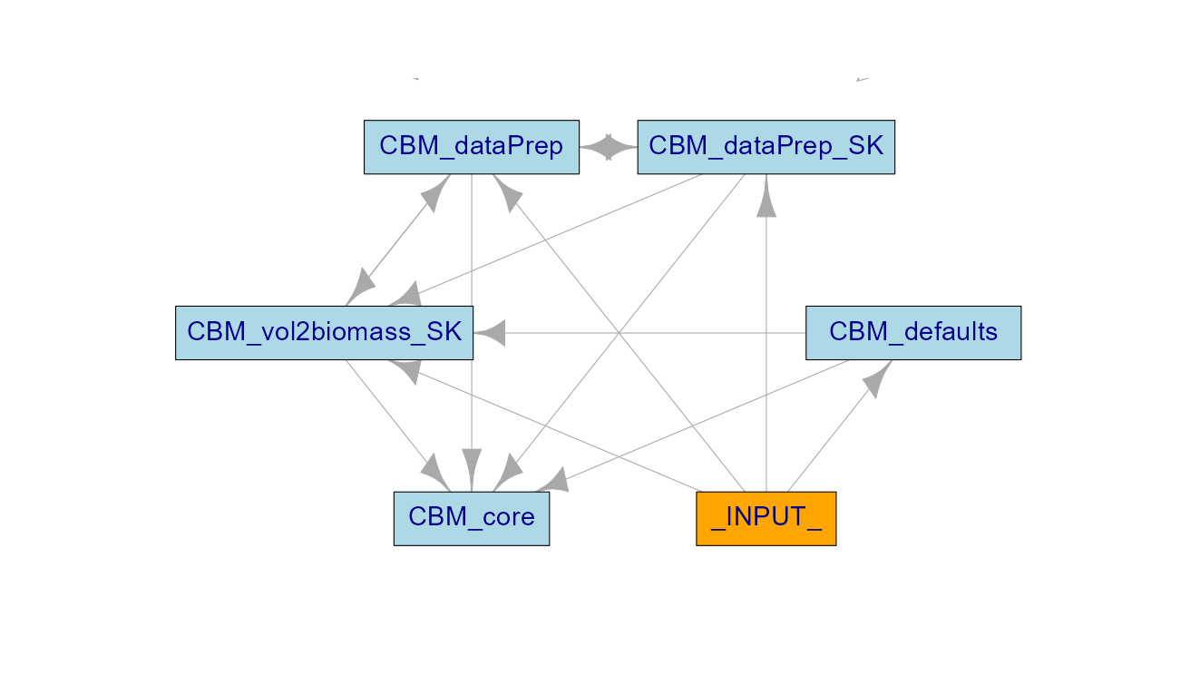
Figure 1: moduleDiagram of spadesCBM
Several core utilities to spadesCBM are provided by the CBMutils package, available on GitHub. The SpaDES platform has a much broader scope than our use of it in spadesCBM. We provide some basic SpaDES definitions here so that users can perform spadesCBM simulations without having to learn all the SpaDES capacities. CBMutils functions used in our example and mentioned in thsi manual will have links to their code and/or documentation. Active development in CBMutils and all spadesCBM modules is underway.
The Carbon Budget Model in SpaDES
The Carbon Budget Model (CBM) was first developed in the early 1990s (Kurz et al. (1993)). Its implementation in a platform for model inter-operability and nimbleness such as SpaDES warrants an overview.
spadesCBM simulates forest carbon dynamics for a given study area based on Canadian-parameterization and user-provided growth and inventory information. Default Canadian parameters are read-in (CBM_defaults), matched to the user-provided information (CBM_dataPrep_SK and CBM_vol2biomass), and this information drives the carbon-transfers through the simulations (CBM_core).
Input requirements
spadesCBM simulations require study area information, age, and leading species of each stand or pixel to simulate on the landscape, and growth information for each stand or pixel. Users can provide this information in various formats which is processed in CBM_dataPrep_SK and in CBM_vol2biomass. We suggest users modify the example provided to represent their study area and inventory information. Each module has a chapter which lists module inputs and outputs.
Pools
There are 14 internal carbon pools in spadesCBM, representing a stand or pixel (Table 1), and 5 pools that take carbon out of the system, products and gas emission to the atmosphere. The carbon transfers are dictated by matrices (available in CBM_defaults) which specify the proportion of carbon moving between two pools (source_pool to a sink_pools). Matrices for growth are populated with the user-provided growth information and are the main change agent in the system, providing carbon input to the stand. Default parameters for biomass and dead organic mater (DOM) turnover, decay, and soil mixing are either at the provincial/territorial, ecozone, or Canada-wide scale (see Table 1 in Kurz et al. (2009)). Note that parameters can easily be modified from their defaults in a spadesCBM simulation. Disturbances matrices representing carbon-transfers during disturbances like fire or harvesting, are available in the defaults (read-in via CBM_defaults) for all managed forests of Canada.
Table 1: Carbon pools in spadesCBM
| Pool | Description |
|---|---|
| Merch | Live stemwood of merchantable size |
| Foliage | Live foliage |
| Other | Live branches, stumps, and small trees |
| CoarseRoots | Live roots ≥5 mm diameter |
| FineRoots | Live roots <5 mm diameter |
| AboveGroundVeryFastSoil | The L horizon comprised of foliar litter plus dead fine roots <5 mm diameter |
| BelowGroundVeryFastSoil | Dead fine roots in the mineral soil <5 mm diameter |
| AboveGroundFastSoil | Fine and small woody debris plus dead coarse roots in the forest floor ≥5 and <75 mm diameter |
| BelowGroundFastSoil | Dead coarse roots in the mineral soil ≥5 diameter |
| MediumSoil | Coarse woody debris on the ground |
| AboveGroundSlowSoil | F, H, and O horizons |
| BelowGroundSlowSoil | Humified organic matter in the mineral soil |
| StemSnag | Dead standing stemwood of merchantable size including bark |
| BranchSnag | Dead branches, stumps, and small trees including bark |
| CO2 | CO2 emitted to atmosphere |
| CH4 | CH4 emitted to atmosphere |
| CO | CO emitted to atmosphere |
| NO2 | NO2 emitted to atmosphere |
| Products | Harvested forest products |
Order of operations
In simulations, disturbances occur before any other carbon transfer. After the disturbances, half of the growth (determined by increments in the user-provided growth curve) is applied followed by the transfers representing DOM turnover, live biomass turnover, an overmature decline compensation if applicable, the 2nd half of the growth, DOM decay, slow decay and slow soil mixing. As previously stated, carbon additions to the system come from the atmosphere (amount determined by growth via user-provided growth curves), and carbon exits the system to the atmosphere or to the forest products sector.
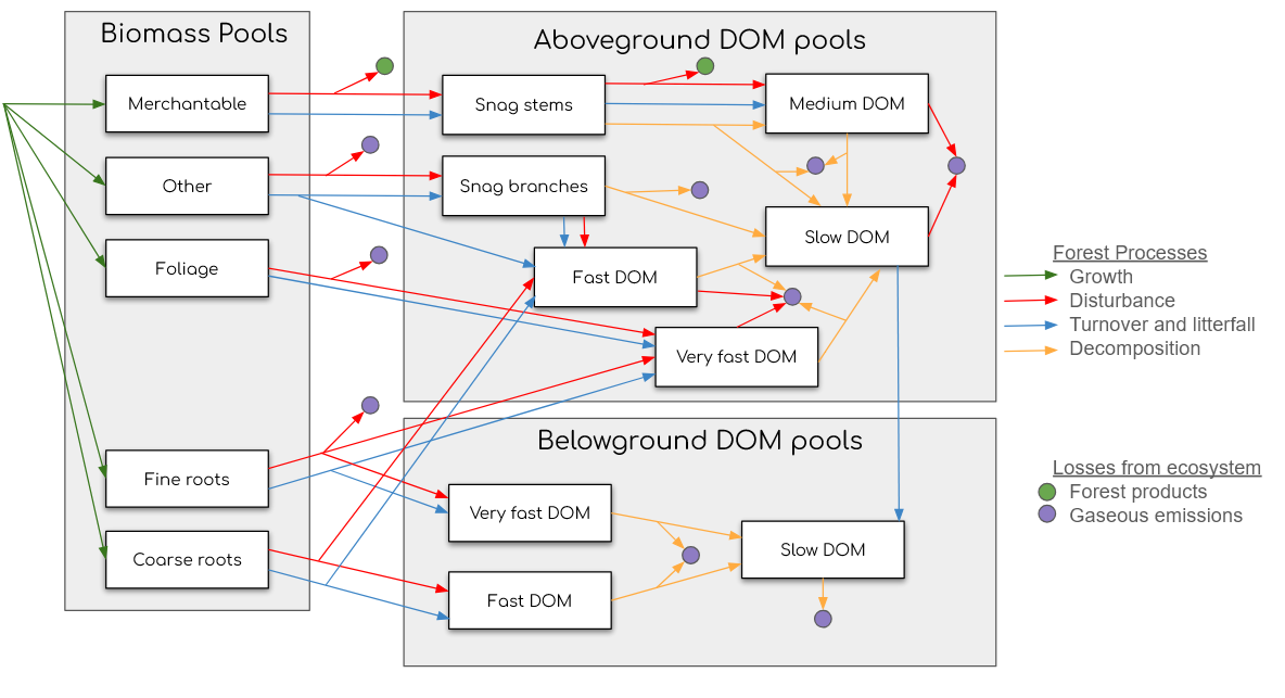
Figure 2: Carbon pools and transfers diagram in spadesCBM
Transfers are proportions of a source pool to sink pools and proportions add up to 1, so no carbon is lost.
Table 2: Types of carbon transfers in spadesCBM
| Carbon Transfers |
|---|
| disturbance |
| half growth |
| domturnover |
| bioturnover |
| overmaturedecline |
| 2nd half of the growth |
| domdecay |
| slowdecay |
| slowmixing |
The spinup function
The amount of carbon below ground in forests is extremely variable and consequently there are few data that can provide this information at scales greater than plot levels. To compensate for this gap in knowledge and data, prior to a simulation, CBM_core completes a process that populates below ground pools. This process is called a spinup and it is the first event in the CBM_core module. The procedure consists of growing and burning forest stand, according to the provided growth curves and default values for fire return intervals (provided in CBM_defaults) until the below ground carbon pool stabilize the aboveground slow (in the soil organic layer) and belowground slow (mineral soil) pools reach a quasi-equilibrium state when the difference between the sum of the pools’ C stocks at the end of two successive rotations is ≤0.1% or reach a predefined number of simulations. Once this state has been reached, one last simulation of the spin-up completes the initialization. In the last simulation the most recent stand-replacing disturbance, as defined by the inventory record, is applied to the stand, and the model grows the forest stand to the current age, also defined in the inventory record. The choice of a fire disturbance to recreate existing conditions matches the historical forest disturbance for most forests in Canada. We consider this procedure a place holder until our knowledge of below ground carbon dynamics improves. Although it will likely be resulting in errors in absolute carbon stocks (see Boisvenue et al. (2022) Appendix 4), these should be systematic errors and we can at least simulate the trends in carbon stocks and fluxes. Research has compared below ground stocks values (Shaw (2008)) and work continues to improve parameters (Hararuk (2017)).