Example: spadesCBM in Saskatchewan

Here we provide an example script to run all managed forests in Saskatchewan between 1985 and 2011. This example is fairly lightweight and most computers should be able to run the simulation.

In this example, we setup the workflow using the SpaDES.project package and current versions of the spadesCBM modules.

Setup

A few things need to be set up the first time running spadesCBM. While the global script below will take care and guide you through most of these, here are some things to note during the initial set up.

Google account

To run the provided example, users need to access some of the data using the googledrive R package (part of the tidyverse family of R packages). During the simInit() (or simInitAndSpades) call, a function to initialize (or initialize and run) SpaDES-based simulations, R will prompt you to either choose a previously authenticated account (if you have previously used googledrive) or to open a browser window and authenticate.

Make sure you give tidyverse read/write access to your files:

Python

The CBM_core module, which is the simulation module of spadesCBM, requires Python >=3.9 and <=3.12.7.

If a suitable version of Python does not already exist on your computer, The reticulate package will be used to install it using the pyenv or pyenv-win.

If you are using a Windows computer with Git installed, the pyenv-win tool will be acquired and managed directly by reticulate. If you are using a Windows computer without Git installed, you will be prompted to allow the pyenv-win tool to be downloaded directly from Github to your local user application data directory (tools::R_user_dir("CBMutils")).

If the Python installation process fails or you would prefer to manually install Python, it can be downloaded directly from python.org/downloads. The calls to Python are for functions from a package called libcbm. Python functions are only used in the CBM_core module. Details on CBM_core module and the Python functions are provided in CBM_core chapter in this manual.

Running the simulation

Here is an R script to run the simulation of forest carbon dynamics in the managed forests of SK from 1985 to 2011, with disturbances as presented in Boisvenue et al. (2016). Depending on your computing capacity, this may take a while, particularly the first time you run it. Subsequent simulations are much faster because of the use of the reproducible::Cache function.

The simulation period can be changed to be shorter, but disturbances raster are only provided for years within the 1985-2011 range in this example.

# set project paths and install packages
projectPath <- "~/GitHub/spadesCBM"
repos <- unique(c("predictiveecology.r-universe.dev", getOption("repos")))
install.packages("SpaDES.project",
                 repos = repos)

# Set simulation period.In this example we start in 1985, and end in 2011
times <- list(start = 1985, end = 2011)

# This is our setupProject call. This creates the model's folder structure, downloads modules, installs and loads needed packages, and sets options.
out <- SpaDES.project::setupProject(
  Restart = TRUE,
  useGit = "PredictiveEcology", # a developer sets and keeps this = TRUE
  overwrite = TRUE, # a user who wants to get latest modules sets this to TRUE
  paths = list(projectPath = projectPath),

  options = options(
    repos = c(repos = repos),
    Require.cloneFrom = Sys.getenv("R_LIBS_USER"),
    reproducible.destinationPath = "inputs",
    ## These are for speed
    reproducible.useMemoise = TRUE,
    # Require.offlineMode = TRUE,
    spades.moduleCodeChecks = FALSE
  ),
  modules =  c("PredictiveEcology/CBM_defaults@main",
               "PredictiveEcology/CBM_dataPrep_SK@main",
               "PredictiveEcology/CBM_vol2biomass_SK@main",
               "PredictiveEcology/CBM_core@main"),
  times = times,
  require = c("reproducible"),

  params = list(
    CBM_defaults = list(
      .useCache = TRUE
    ),
    CBM_dataPrep_SK = list(
      .useCache = TRUE
    ),
    CBM_vol2biomass_SK = list(
      .useCache = TRUE
    )
  ),

  #### begin manually passed inputs #########################################
  ## define the  study area.
  masterRaster = {
    mr <- reproducible::prepInputs(url = "https://drive.google.com/file/d/1zUyFH8k6Ef4c_GiWMInKbwAl6m6gvLJW",
                                   destinationPath = "inputs")
    mr[mr[] == 0] <- NA
    mr
  },

  disturbanceRastersURL = "https://drive.google.com/file/d/12YnuQYytjcBej0_kdodLchPg7z9LygCt",

  outputs = as.data.frame(expand.grid(
    objectName = c("cbmPools", "NPP"),
    saveTime = sort(c(times$start, times$start + c(1:(times$end - times$start))))
  ))
)

# Run simulation
simMngedSK <- SpaDES.core::simInitAndSpades2(out)

Viewing results

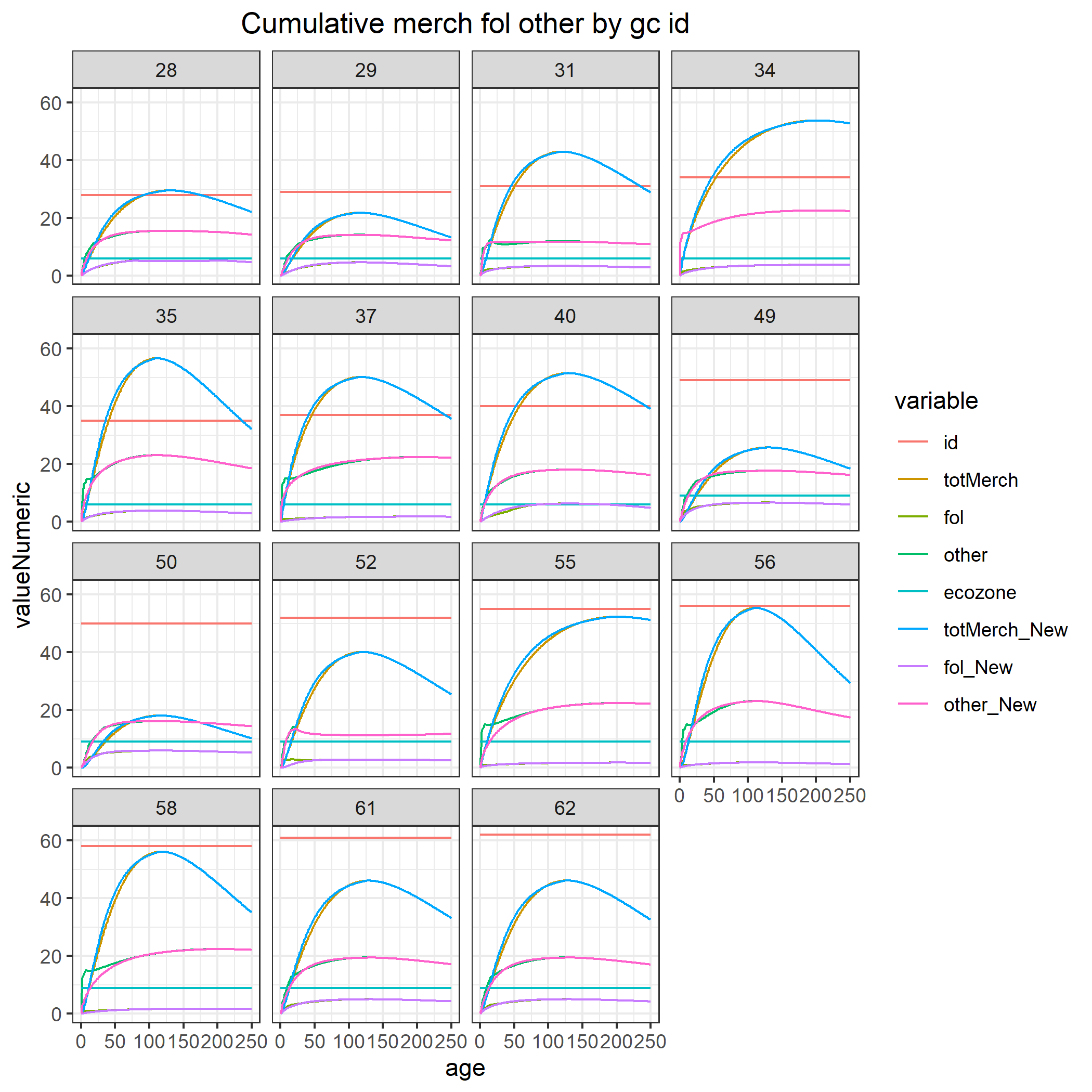
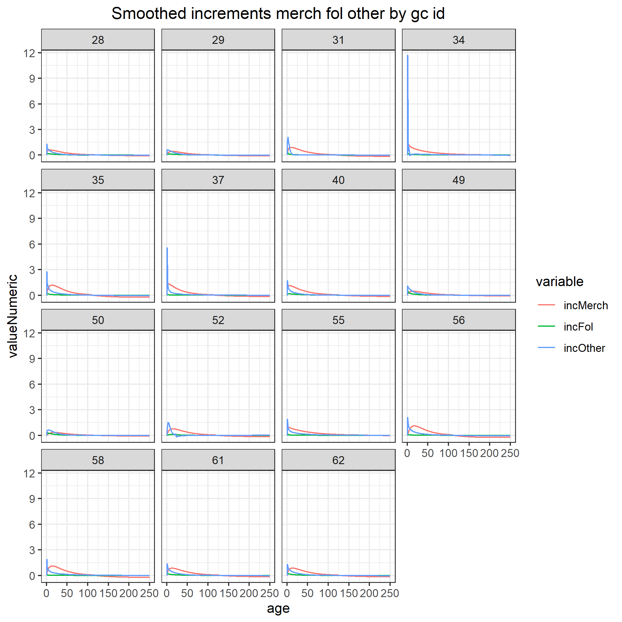
Once the simulation has run, we can view our results. Some of these are saved as files in the outputs folder created in the project’s directory. If kept as the default in the global script above, these can be found here: ~/GitHub/spadesCBM/outputs. You should be able to see .rds files for cbmPools and NPP for each simulated year, as well as various growth curve and increment related figures from CBM_vol2biomass_SK shown below.

The simMngedSK object in R is the resulting simlist of our simulation. CBMutils offers a few plotting functions to help visualize basic results using our simlist.

# Yearly forest products and emissions for each simulation year
carbonPlot <- CBMutils::carbonOutPlot(
  emissionsProducts = simMngedSK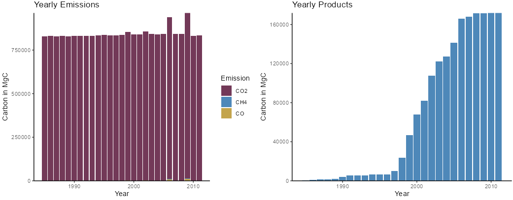$emissionsProducts
)

# Proportions of carbon in above and below ground compartments
barplot <- CBMutils::barPlot(
  cbmPools = simMngedSK$cbmPools
)

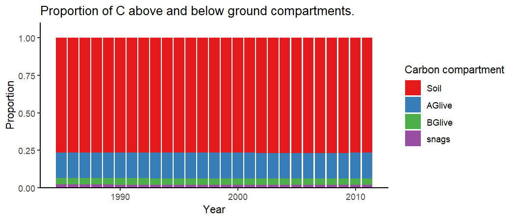
# Map of pixel-level average NPP
NppPlot <- CBMutils::NPPplot(
  cohortGroupKeep = simMngedSK$cohortGroupKeep,
  NPP = simMngedSK$NPP,
  masterRaster = simMngedSK$masterRaster
)

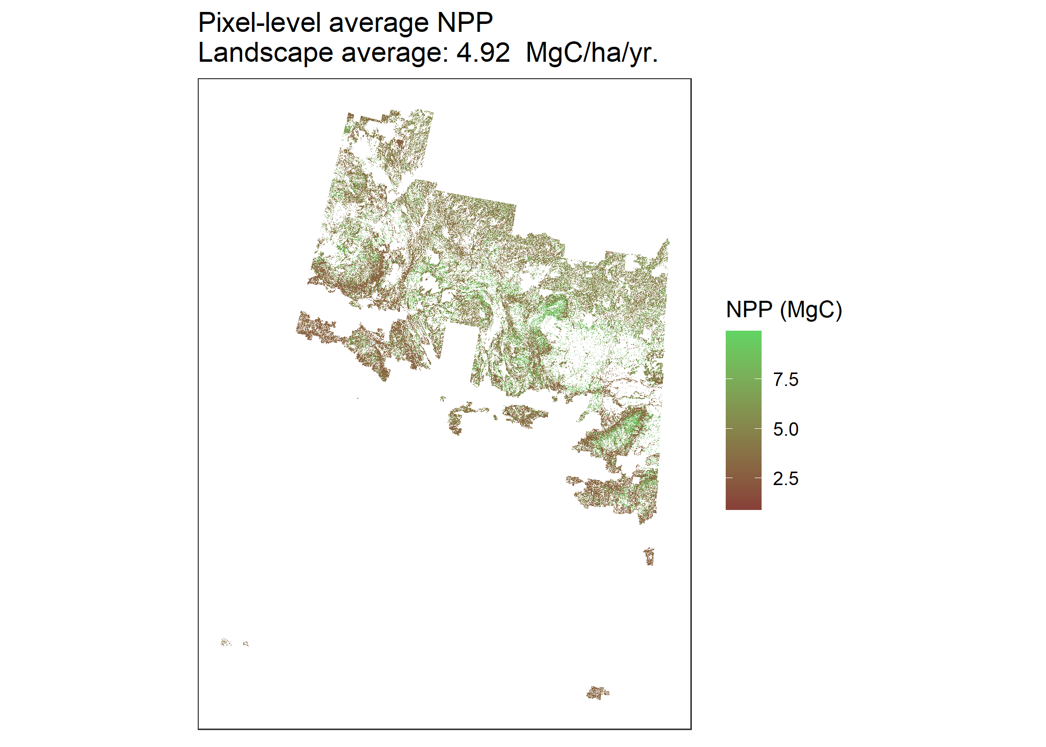
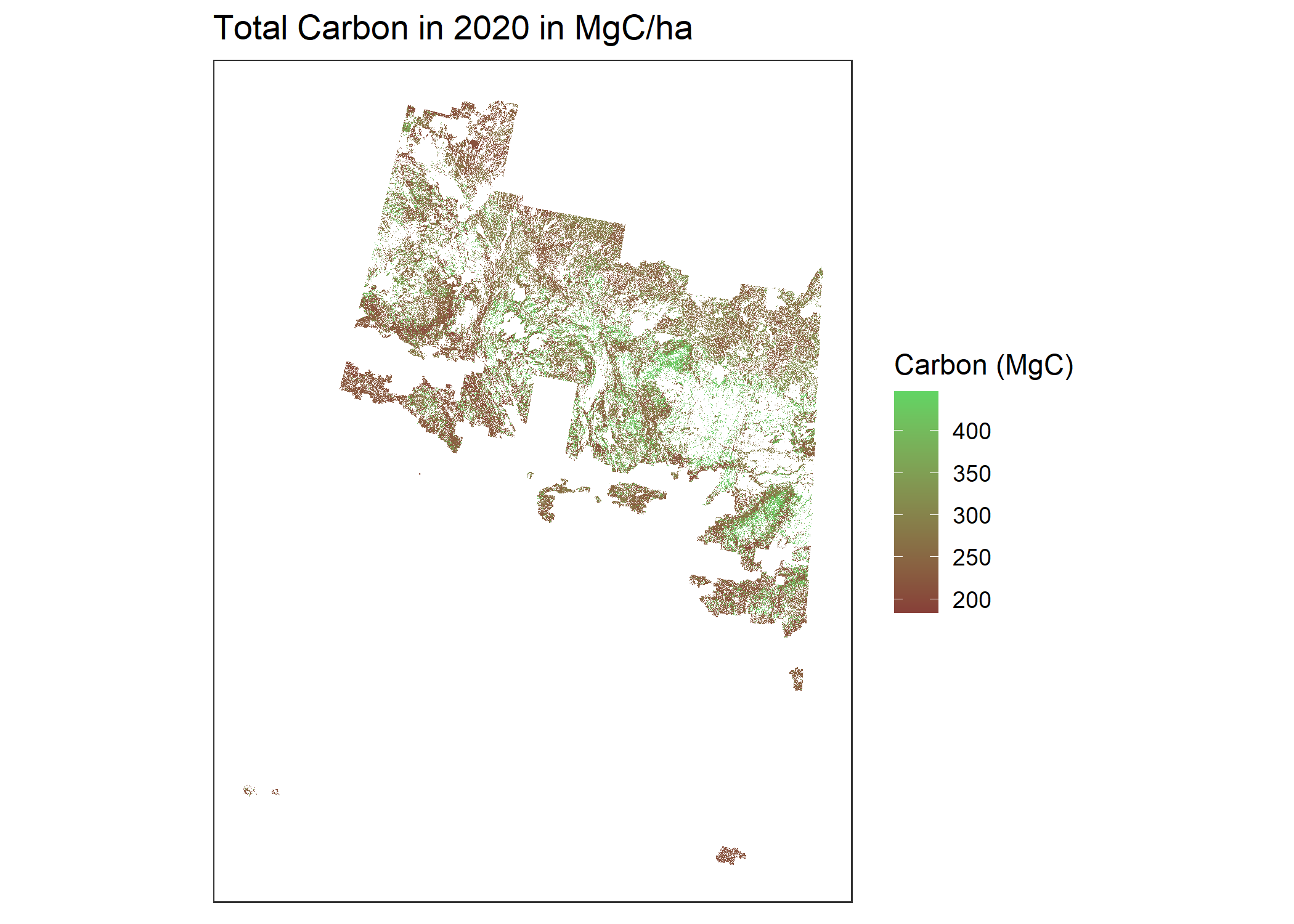
# Map of total carbon per pixel for a simulation year
spatialPlot <- CBMutils::patialPlot(
  cbmPools = simMngedSK$cbmPools,
  years = 2000, # set simulation year 
  masterRaster = simMngedSK$masterRaster,
  cohortGroupKeep = simMngedSK$cohortGroupKeep
)

4 CBM_core

References